

nvmath-python (Beta) 是一個開源 Python 庫,為 Python 程序員提供對 NVIDIA CUDA-X 數學庫的高性能數學運算訪問。nvmath-python 既提供底層庫的低級綁定,也提供更高級別的 Python 抽象。它可與 PyTorch 和 CuPy 等現有 Python 軟體包進行互操作。
在本文中,我將展示如何在 nvmath-python 中將 結語 與矩陣乘法結合使用。結語是可以與正在執行的數學運算(如 FFT 或矩陣乘法)融合的運算。可用的結語涵蓋了大多數常見的深度學習計算。我通過實施簡單神經網路的常見正向和反向傳遞運算來演示其用法。
要安裝 nvmath-python,請 按照安裝說明 操作。
使用 RELU_BIAS 後記優化正向傳遞
在本節中,我將演示如何使用 epilogs 實現簡單線性層的前向傳遞。此層首先將輸入向量乘以權重矩陣,然後向生成矩陣的每個元素添加偏差,最後應用 ReLU 激活函數。
ReLU 是修正線性單元的簡稱,是一種常用的激活函數,可以在保持正值不變的同時將負值替換為 0。
在矩陣運算方面,該層可以表示為:

在方程中,以下定義成立:
- 是一批形狀為的輸入向量 :
- 是層的輸入數量。
- 是批量大小。
- 是形狀的權重矩陣 :
- 是層的輸出數量。
- 是其輸入的數量。
- 是長度為 的偏置向量,將其添加到生成矩陣的每一列中。
假設您的輸入、權重和偏差為 CuPy 數組:
num_inputs, num_outputs = 784, 100batch_size = 256weights = cupy.random.rand(num_outputs, num_inputs)bias = cupy.random.rand(num_outputs)x = cupy.zeros((num_inputs, batch_size)) |
在最基本的版本中,您可以通過使用 nvmath-python 計算 ,然後手動處理偏差和 ReLU 來實現此線性層,如下代碼示例所示。
在本示例中,我使用 nvmath.linalg.advanced.Matmul -class.html」 rel=」follow noopener」 target=」_blank」>有狀態 API ,其中您可以將初始化和規劃與乘法的實際執行分開。當您必須執行多個類似的乘法運算時,我推薦這種方法,因為它可以讓您分期償還規劃的初始成本。有關 Matmul 的更多資訊,請參閱 nvmath.linalg.advanced.Matmul。
mm = Matmul(weights, x)mm.plan()def forward(): y = mm.execute() y += bias[:,cupy.newaxis] y[y < 0] = 0 return y |
要提高代碼的性能,請利用 RELU_BIAS epilog 在單個融合的 cuBLAS 操作中執行所有三個操作。這個結語首先將偏差添加到乘法結果中,然後應用 ReLU 函數。
您可以使用 Matmul.plan 方法的 epilog 參數指定結語。一些結語(包括 RELU_BIAS)會接收額外的輸入,可在 epilog_inputs 字典中指定。有關結語的更多資訊,請參閱 nvmath.linalg.advanced.Matmul 。
from nvmath.linalg.advanced import MatmulEpilogmm = Matmul(weights, x)mm.plan(epilog=MatmulEpilog.RELU_BIAS, epilog_inputs={"bias": bias})def forward(): y = mm.execute() return y |
正如我稍後解釋的那樣,要通過 ReLU 函數進行反向傳播,您必須知道向 ReLU 的哪些輸入為正、哪些為負。此輔助資訊稱為 ReLU 掩碼 ,可通過 RELU_AUX_BIAS 後記獲得。
當使用帶有輔助輸出的結語時,Matmul.execute 將返回一個包含實際結果和輔助輸出字典的元組。在 RELU_AUX_BIAS 的情況下,輔助輸出字典只有一個鍵 relu_aux,其中包含 ReLu 掩碼。該掩碼是位編碼的,可能難以讀取,但在向後傳遞期間,有專門的結語可以為您執行此操作。
from nvmath.linalg.advanced import MatmulEpilogmm = Matmul(weights, x)mm.plan(epilog=MatmulEpilog.RELU_AUX_BIAS, epilog_inputs={"bias": bias})relu_mask = Nonedef forward(): global relu_mask y, aux_outputs = mm.execute() relu_aux = aux_outputs["relu_aux"] return y |
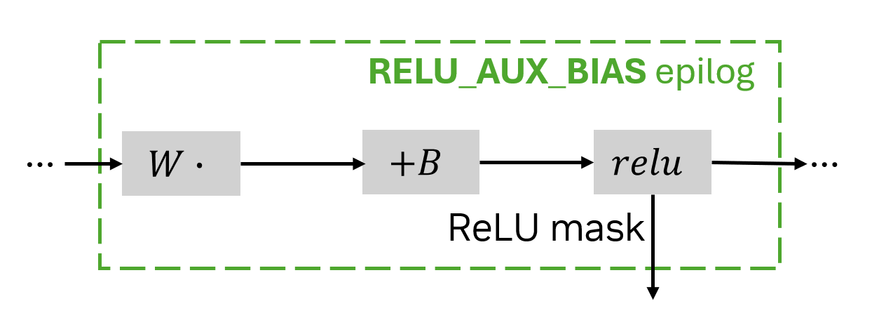
使用 RELU_AUX_BIAS epilog 的實現速度比其樸素的實現要快,從而顯著提升性能。
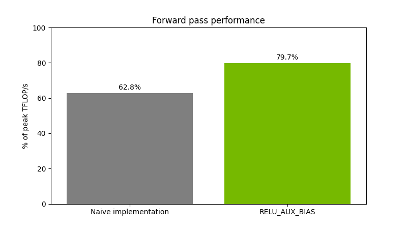
圖 2 顯示了對大小為(65536,16384)(16384,8192)的 float16 矩陣執行矩陣乘法運算,然後執行偏加和 ReLU 運算。性能在 NVIDIA H200 GPU 上進行測量。
使用 DRELU_BGRAD 後記優化反向傳播
在神經網路的反向傳播過程中,損失函數相對於輸出的梯度會反向傳播到網路層,以計算每個參數的梯度。
直觀地說,對於每個操作,當其輸出對損失的影響已知時,就有可能確定其輸入和參數(例如權重矩陣中的值)如何影響損失。有關更多資訊,請參閱 反向傳播 。
在這一部分,我假設有多個線性層堆疊在一起。我對通常被認為屬於不同層的操作序列實施反向傳播:添加偏差、應用 ReLU 以及乘以權重。
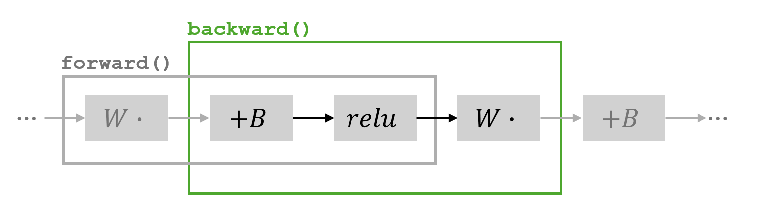
forward 中實施的操作以及 backward 中涵蓋的部分
讓 作為前面顯示的網路部分的輸入,並分別通過 、 和 顯示中間結果:
在反向傳播中,當您知道 loss function 是如何受 (即 )影響時,即可計算相對於其他參數的梯度。如需詳細瞭解用於計算梯度的公式的推導,請參閱 Automatic Differentiation 和 Neural Networks 。
- ,其中 為負值,,其中 為非負值(ReLU 掩碼包含此資訊)
- 是 ,按批量維度求和
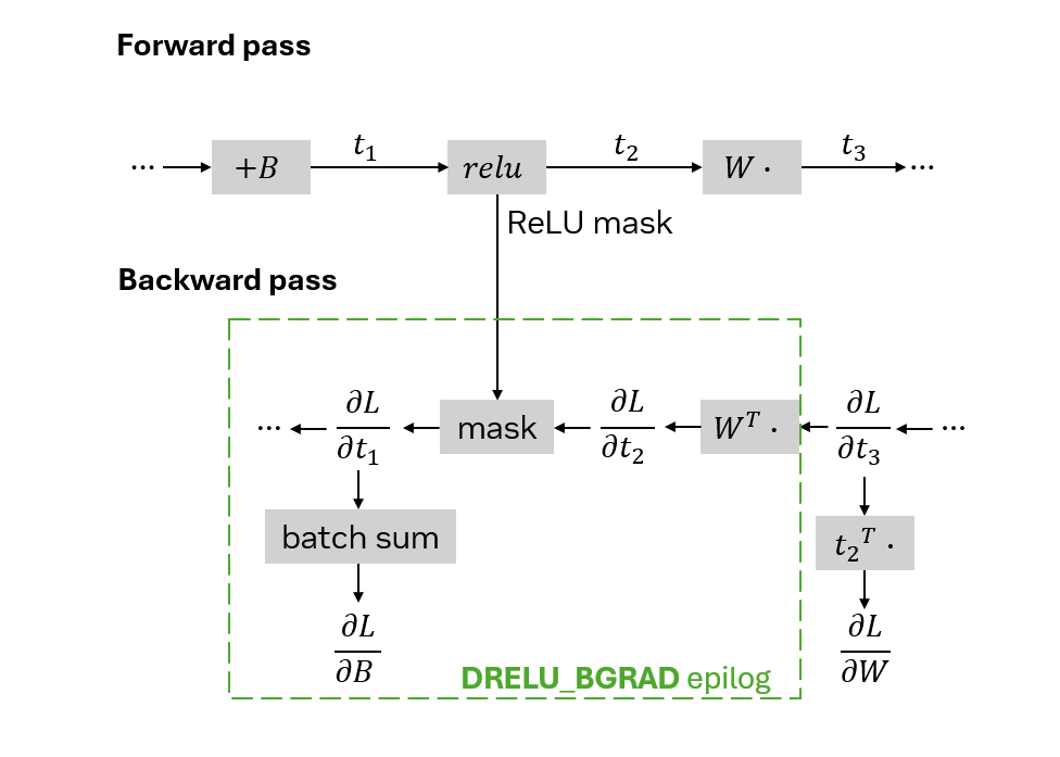
計算 和 所需的運算可以通過使用僅用於矩陣乘法的 Matmul,然後手動處理掩碼和批量和來簡單實現。
mm = Matmul(weights.T, grad)mm.plan()def backward(): grad_t1 = mm.execute() grad_t1[mask] = 0 # assuming that `mask = (t1 < 0)` grad_bias = cupy.sum(grad_t1, axis=1) return grad_t1, grad_bias |
要優化您的向後傳遞,請使用 DRELU_BGRAD 後記。假設梯度 在 CuPy 數組 grad 中可用。DRELU_BGRAD 的 epilog 需要一個輸入 relu_aux,其中包含從 RELU_AUX_BIAS 的 epilog 返回的掩碼。它將此遮罩應用於乘法結果。它還會返回一個輔助輸出,其中包含結果的逐列總和,恰好是 。
mm = Matmul(weights.T, grad)mm.plan(epilog=MatmulEpilog.DRELU_BGRAD, epilog_inputs={"relu_aux":relu_mask})def backward(): grad_t1, aux_outputs = mm.execute() grad_bias = aux_outputs["drelu_bgrad"] return grad_t1, grad_bias |
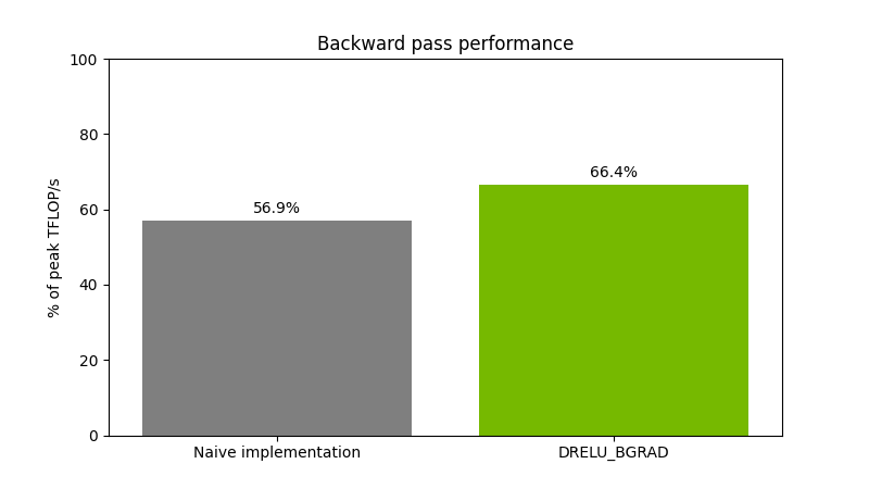
圖 5 顯示了對大小為(65536,16384)(16384,8192)的 float16 矩陣執行矩陣乘法運算,然後應用 ReLU 掩碼和偏差梯度計算。該性能在 NVIDIA H200 GPU 上進行了測量。

 WeChat
 Profile